Exploring Variance in N-Step Actor-Critic Methods

David Biertimpel, Claartje Barkhof, Vicky Foing & Alex Lindt

*University of Amsterdam | October 2019

Lunar_landar

Figure 1: Behavior in Lunar Lander environments

Introduction

Imagine two athletes training for a competition. The first athlete’s coach is a master of his trade, but due to his advanced age teaches techniques which are consistent but slightly antiquated. The second athlete is coached by a rising star just graduated from the academy. Although her instructions fit exactly to the modern sport, she is still inconsistent in her decisions because of her lack of experience. Which athlete will perform better in the competition? This question reflects the bias-variance trade-off in reinforcement learning. While the first athlete exactly learns the biased strategy of his coach, the instructions the second athlete receives have high variance.

In this blog article, we investigate bias and variance in actor-critic methods by comparing different n-step bootstrapping returns ranging from TD(0) to Monte Carlo across multiple environments. The core of actor-critic methods is the policy gradient which recently achieved great success in various control tasks such as 3D locomotion 1, playing video games 2 or solving a Rubik’s cube 3. The biggest advantages of policy gradient methods are that they are predestined for continuous action spaces, implicitly learn stochastic policies, and have overall good convergence properties. However, policy gradient methods have also proven to show high variance in many aspects, such as performance over multiple runs (different random seeds), sensitivity to fine changes in hyperparameters, and low robustness to unexpected changes in the environment 4, 5. This makes policy gradient methods not always reliable and complicates the reproduction of results. The most obvious source of variance is the variance in sampled trajectories and therefore in the accumulated rewards (return) the agent receives during these trajectories. Here we have a strong incentive to regularize this variance as it hinders accurate gradient estimation, which consequently slows learning. This is why, over the next sections, we investigate various n-step estimates of the return ranging from high bias and low variance TD(0) to low bias and high variance Monte Carlo.

Policy Gradient Methods

But first, before we dive deep into the topic, let’s refresh our knowledge about reinforcement learning and policy gradients. In reinforcement learning our goal is to maximize the future return $G$ the agent receives by interacting with the environment under a specific policy $\pi$ :

$J = E_{\tau} \bigg[ G(\tau) \bigg]$

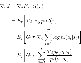
In policy gradient methods we directly model the policy with a parameterised (often nonlinear) function $\pi_{\theta}$ such as a neural network and aim to perform gradient updates in the direction of the maximal return. In order to do this, we must take the gradient of return which we achieve by using the following identity:

form2

Reinforce

This results in the most basic policy gradient method called REINFORCE. The intuition here is that we make actions connected to a high return more likely. When looking at the last bit of this derivation we also see explicitly that we are correcting for the frequency with which the policy selects actions.

Without getting lost in further mathematical derivations, we can easily imagine that the return of the full trajectory $G(\tau)$ has high variance between episodes, due to stochasticity of the environment’s dynamics and the policy, and that we might want to introduce different estimates of the return. One prominent method to reduce variance is subtracting a baseline from the return, which is then called REINFORCE with baseline. A good candidate for the baseline is the state-value function $V_{\pi}(S)$ , which describes how much reward the agent is expected to receive from state $S$ onward when following policy $\pi$ . Similar to our policy, we can also estimate $V_{\pi}(S)$ with a nonlinear function approximator like a neural net. The intuition behind subtracting $V_{\pi}(S)$ from the actual return is that we separate the action quality from the quality of the current state. This return estimate suffers less from variance, but introduces bias, since $V_{\pi}(S)$ is randomly initialized and does not reflect the true state-value in the beginning.

Instead of considering the full return of the trajectory, we can also calculate the TD-target form3 which becomes the TD-error when combined with the baseline $V_{\pi}(S)$ . This reduces the variance to a minimum as we are only looking at the next step the agent takes. The intuition for this return estimate is that we are happily surprised if the TD-error is positive, since we received more reward than expected and thus increase the probability of the corresponding action. Conversely, in the case of a negative TD-error we receive less reward than expected and disappointedly lower the probability of the corresponding action.

A different instantiation of the TD-error can be achieved by using the action-value function $Q_{\pi}(S, A)$ . The action-value function describes future reward the agent can expect when taking action $A$ in state $S$ and follow policy $\pi$ afterwards. The corresponding TD-error is form3 . For the same reasons as $V_{\pi}$ , $Q_{\pi}$ is also a biased estimate of the action-value function when approximated via bootstrapping.

Actor-Critic Methods

By using the TD-error instead of the full return, we finally arrive at the methods on which we mainly focus in this article: actor-critic methods. In the case of actor-critic methods we use the $V_{\pi}$ or $Q_{\pi}$ estimates not only as a baseline, but also for bootstrapping (updating the estimate of $V_{\pi}$ or $Q_{\pi}$ with another estimate of $V_{\pi}$ or $Q_{\pi}$ ). This bootstrapping introduces a significant bias, which helps reduce variance in the updates and therefore should stabilize and accelerate learning. Actor-critic methods have their name from combining a parameterized policy $\pi_{\theta}$ that decides which actions to take (the actor) and an estimate of $V_{\pi}$ or $Q_{\pi}$ which provides an opinion about the quality of current actions and/or states the agent ends up in (the critic). So the actor tells us how to act and the critic tells us how well we are acting. As already indicated above, the version of actor-critic we are going to focus on is where the TD-error is used as the critic estimate. This version is called advantage actor-critic because it determines the advantage in the return from taking the action in the current state compared to the expected return in that state.

Policy Gradient Theorem

Perhaps you are wondering now how on earth we can seamlessly exchange $G$ with all these different return estimates. This is possible because of the Policy Gradient Theorem, which states that for any differentiable policy $\pi_{\theta}$ , for any policy objective function $J$ the policy gradient is:

form6

where $\Psi_t$ is a placeholder for different return estimates. The derivation of this theorem is actually quite straightforward and is nicely explained in Schulman’s General Advantage Estimation (GAE) paper 1 or for people who prefer visual input in Hado van Hasselt’s deepmind lecture on Policy Gradients and Actor-Critics at UCL.

N-step bootstrapping

Now we heard about quite some strategies to choose either a biased (TD-error) or high variance estimate (Monte-Carlo in REINFORCE), however, the choice has been quite binary so far. In order to be able to study the trade-off between bias and variance it would be nice to have some estimates between both extremes. Here n-step returns enter the ring. Instead of bootstrapping with the estimated state-value of the next state as in the TD-error before, we also can observe a longer chain of rewards before plugging in the estimated state value. The state value it plugs in might be n steps away, which makes up for the name n-step actor-critic methods. N-step returns can be naturally integrated the actor-critic methods described above, as we just have to our TD-target. Where we had form3 before, we can now plug in form5 .

If we have $n=\infty$ we get exactly the full Monte-Carlo return $G$ from REINFORCE, by contrast if we leave $n=1$ the method equals the previously described TD-error with a one-step look ahead.

Based on the theory outlined above, we hypothesise that by tuning the n-step, ranging from one-step actor-critic (high bias) to REINFORCE with baseline (high variance), we can tune the bias-variance trade-off in order to pick a sweet spot dependent on each environment. In other words, we will investigate if different values for n will be beneficial for different algorithm and environments.

Methods

To make the comparison between different methods as fair as possible we implement them all following the same pseudocode. The general pseudo-code can be laid out as follows:

# INITIALISE EXPERIMENT
actor_θ, critic_w ← parameterised functions instantiated as neural networks
ɑ_θ, ɑ_w ← step size for actor and critic respectively

# EXPERIMENT LOOP
for each episode in max_episodes:
    
    # INITIALISE EPISODE
    state ← start state of environment
		𝚿_record, log_probabilities, states, rewards ← []
    
    # EPISODE LOOP
    for each step in episode t=0,1,...,T:
        policy ← actor_θ(state)
        log_probabilities ← log(policy)
        next_state, reward ← environment_step(sample(policy))
        rewards ← rewards + reward
        states ← states + state
        𝚿_record ← 𝚿_record + 𝚿_function(next_state, states, rewards, critic)
        state = next_state
    endfor
   
   	# UPDATE PARAMETERS
   	loss_actor ← mean( - log_probrobabilities * 𝚿  									  																		- log_probabilities.entropy() * 0.01) # polict gradient
    loss_critic ← mean(𝚿**2) 																# mean squared error
    θ ← θ + ɑ_θ * loss_actor
    w ← w + ɑ_w * loss_actor

endfor

The different instantiations of $\Psi$ are as follows:

Algorithm	𝚿_function
REINFORCE with baseline	$\Psi_{t} \leftarrow G_{t} - \hat{v}(S_{t},w)$
Advantage Actor-Critic (1-step)
Advantage Actor-Critic (n-step)
Q Actor-Critic (1-step)
Q Actor-Critic (n-step)

In contrast to how the actor-critic procedure is described in Sutton & Barto 6, we do not update our models after every time step in the environment but do a batch update at the end of every episode. This stabilizes our gradients and corresponds to description in related papers and professional implementations online 7. Inspired by the A2C algorithm 8 we introduce an entropy term in the actor loss reflecting the entropy of the Categorical distribution over the actions. This term flattens out the action probabilities and enforces exploration.

Experiments

Environments

To test our hypothesis we select three control tasks from the OpenAI’s Gym with different characteristics.

Cartpole

In this game the goal is to balance a pole on a cart. By moving left and right (a discrete action space) one should try to manage keeping the pole upright. The game is over when the pole drops (more than 15 degrees from being upright) or when the cart moves too far off the track in either direction (measured as 2.4 units). The game ends naturally when the pole is balanced for 200 time steps. A reward of +1 is granted for every step that the pole is in the air. The cartpole environment promises us, with its straightforward state and action space, reliable results, such that it should serve as a stable baseline to compare our different methods.

Lunar Lander

In the Lunar lander environment, one has to land a spaceship in between two flags as smoothly as possible. If the spaceship crashes, it receives a reward of -100 and if the spaceship lands smoothly, it receives a reward of +100. The agent has the choice of four actions: Do nothing, Fire left engine, Fire down engine, and Fire right engine. There are additional conditions that influence the agent, such as small punishment (-0.3) for firing the main engine, a small reward (+10) each time a leg touches the ground, wind affecting the orientation of the ship, and a changing landscape. The Lunar Lander environment is a bit more complex as the cartpole both in terms of the reward structure and the fact that the environment slightly changes over different episodes. It is thus interesting to see if our agents will be able to adapt to that.

Mountain Car

In Mountain-Car-v0 one has to try to move a little car up onto a hill. The landscape is a part of a cosine curve of which the highest point is the hill. To reach the top of the hill the car has to gain momentum by driving up and down both slopes alternatingly, since its engine is not strong enough to drive up the hill at once. The version of the game we use consists of a discrete action space {left, right}. For every time step the player did not reach the goal yet a -1 reward is returned, so the is incentivised to reach the hill as fast as possible. An interesting property of this environment is that the agent first needs to reach the goal by random exploration before getting the positive reward that allows learning the optimal policy. Due to the requirement of stochasticity, we expect high-variance agents to perform better.

Experimental set-up & metrics

For each environment, we run experiments with 9 configuration: Reinforce and four versions of each actor-critic algorithm (n=1,n=2,n=4,n=8). Each configuration is run five times, using the same five random seeds. To analyze performance, we store the episode durations, cumulative reward, actor losses, and critic losses, and average across the five runs. These metrics track how quickly and accurately each algorithm learns the reward structure of the environment, which will provide insights into bias and variance.

Architecture & hyper parameters

All algorithms are implemented using two neural networks, one to represent the Policy estimate and one to represent the Value estimate.

The hyperparameters are as follows:

Hyper parameter	Setting
Learning rate	7e-4
Number of episodes	1000
Discount factor	0.99
Number of hidden nodes	two layers of 64 nodes
N-step values	[1,2,4,8]
Number of runs	5
Random seeds for runs	[43,44,45,46,47]

We select these hyperparameters based on experiments from literature as well as some hyperparameter optimization experiments of our own. To ensure fair comparisons, we keep the values the same for all configurations.

Results

Overall performances

First we look at the overall performances of our implemented methods and see how they compare to our baseline algorithm REINFORCE with baseline.

Cartpole

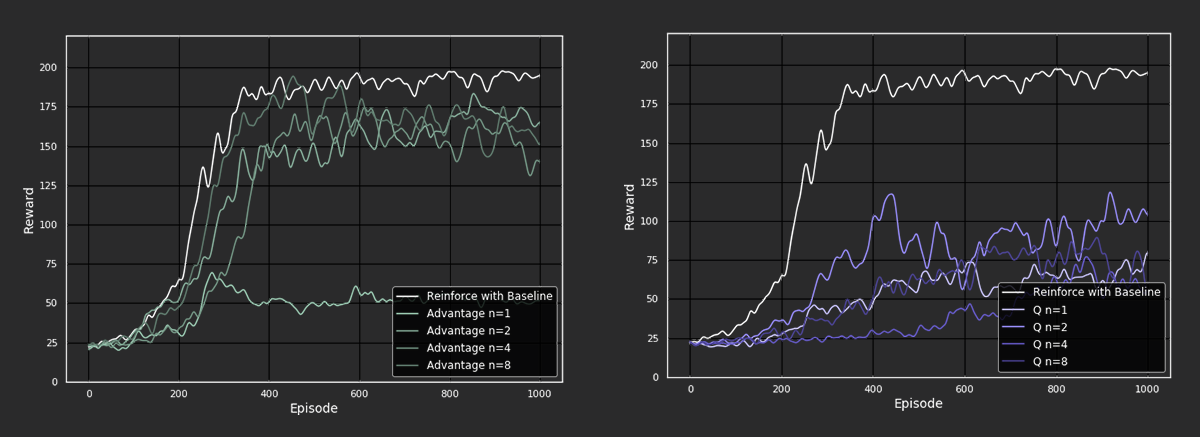
Figure 2: Performance of the different algorithms on the Cartpole environment

From the above plots, it is evident that REINFORCE with baseline outperforms the actor-critic methods, consistently reaching rewards close to 200 (maximum score) after about 300 episodes. For advantage actor-critic, the performance seems to increase as the n-step value increases. Interesting to note is that the performance for n-step values greater than 1 achieve similar rewards as REINFORCE with baseline, close to 175 after 300 episodes. However, the agent where n = 1 falls out of line and and stagnates after 250 episodes.

When looking at the Q actor-critic agents we see a different picture. Here we cannot even say that with increasing n-step the performance of the agents improves, as we observe the best behavior from the n = 2 agent. Overall, the agents do not come close to the performance of the advantage actor-critic agents. A possible reason for this could be that we perform the Q-learning update while bootstrapping ( form11 ) and thus introduce an off-policy aspect into an algorithm that is essentially on-policy.

Lunar Lander

LL_n8

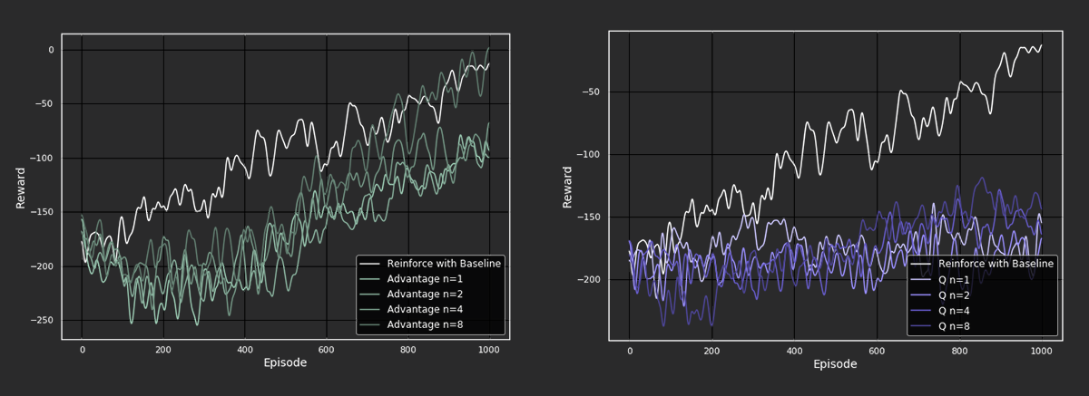
Figure 3: Performance of the different algorithms on the Lunar Lander environment

For the Lunar Lander environment, we also see that REINFORCE with baseline outperforms most of the actor-critic methods. In general, the advantage actor-critic methods show a similar performance as REINFORCE with baseline, improving steadily throughout training. In contrast, the Q actor-critic methods do not improve much throughout the 1000 episodes. Again, the advantage actor-critic methods improve as the n-step increases while the Q actor-critic methods do not. What is exciting in the Lunar Lander environment is that at the end of the training, the advantage actor-critic with the highest n-step value, 8, eventually outperforms REINFORCE with baseline, reaching a reward of 0. This suggests that we have found a sweet spot for this particular experiment, where bootstrapping is better than calculating the full return.

Mountain Car

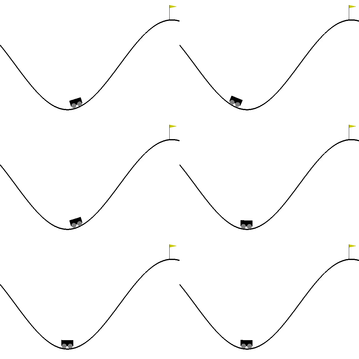general_cartpole Figure 4: Behavior in Mountain Car environment by Q actor-critic (n-step=1)

After a considerable amount of parameter tuning and after running all of our described agents in the Mountain Cari environment, our implementation could not solve the Mountain Car a problem. For reasons we can only speculate about, the agent did not manage to explore enough to reach the top a single time. We assume that because policy gradient methods are on-policy and the exploration is determined by the distribution over actions, the evenly distributed reward of -1 is not enough to enforce enough exploration. Most of our agents perform as shown in the gif above.

Comparing random seeds

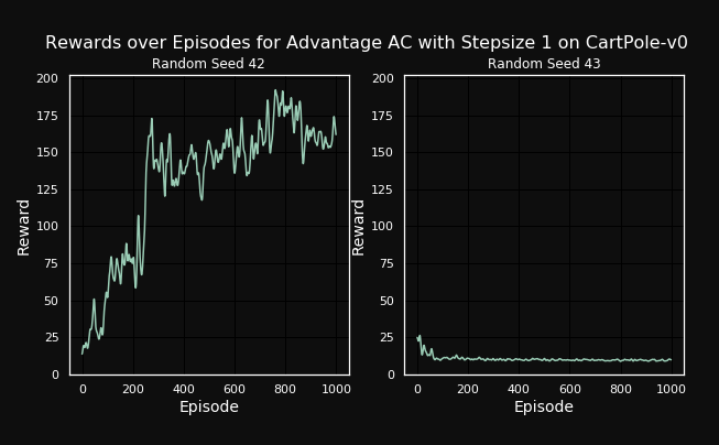random_seed Figure 5: Performance of one step Advantage Actor-Critic on cartpole environment with different seeds

To illustrate the variance over the several runs previous sections, we will now look at two completely identical agents living in the same environment, where the only difference is the selected random seed. While the left agent solves the task almost perfectly reaching the maximum possible reward (not visible due to smoothing), the right agent fails horribly by ranging between 5 and 10 reward over the whole episode. This shows how dependent policy gradient methods are on having a good initialization. In this case we further see another disadvantage of policy gradient: a bad policy leads to bad data. So if the agent behaves suboptimally after some wrong updates in the policy space, the collected data will also be suboptimal. In some cases this can lead to the agent not being able to recover from that.

Variance-bias debate

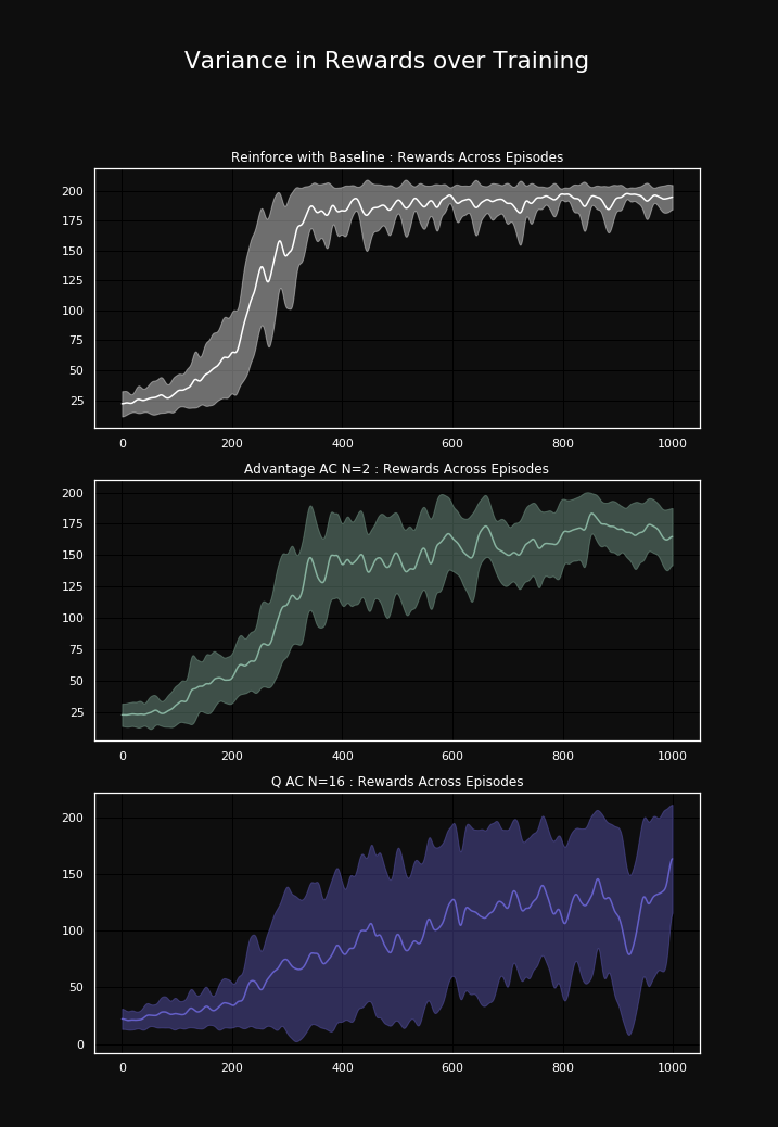variance_rewards_MC_A_Q Figure 6: Cumulative rewards plotted with variance over 5 runs during training for different algorithms

For the experiments of this section we picked the most successful n-step value for advantage actor-critic and Q actor-critic respectively and compared those versions to our baseline algorithm. The experiments are done in the CartPole-v0 environment.To understand the differences of our approaches with regard to the bias-variance tradeoff, we take a closer look at the variance of the rewards and losses they obtain while training. The first figure shows the variance in rewards over the course of training. For REINFORCE with baseline, we can see that the rewards have overall the lowest variance and that the variance is highest in the beginning and gets less over the training. This means that it has learned optimal behavior, which is likely due to the fact that the environment is so simple. In contrast, for Advantage actor-critic and especially for Q actor-critic we see that the variance in rewards is generally higher and also gets higher over training. Both algorithms are less stable in their performance than the REINFORCE with baseline. It is apparent that Q actor-critic is more instable than the Advantage actor-critic in general. Even if it occasionally ‘solves’ the environment in later training steps, obtaining close to the maximum reward of 200, it does obtain rewards of down to 20 at the same time. The Advantage actor-critic, even if more stable that the Q actor-critic, does not work as reliable as the REINFORCE with baseline. Although it achieves comparatively constant rewards between 150 and 200 in the later training steps, it seems to never fully converge to the optimal policy. We interpret this as an expression of the bias of the Advantage actor-critic algorithm, as the known unbiased REINFORCE with baseline does not show this behavior.

Though it achieves a decent performance, Advantage actor-critic does not achieve the same optimal performance as REINFORCE with baseline, which could be due to bias.

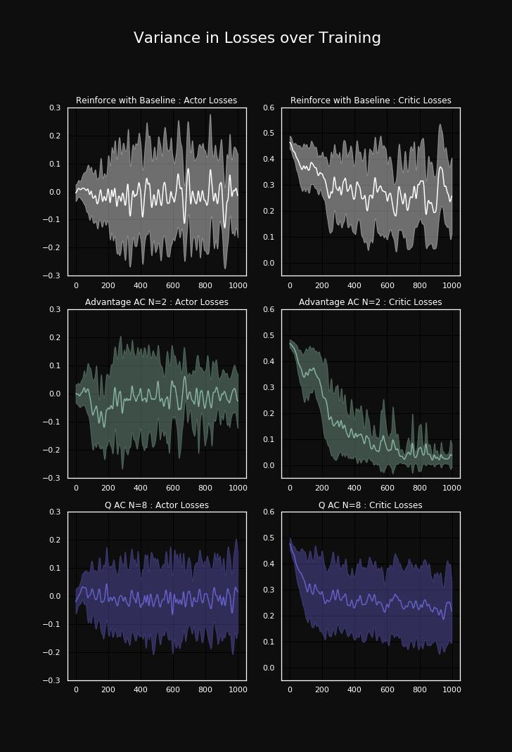variance_losses_MC_A_Q Figure 7: Actor and critic loss plotted with variance over 5 runs during training for different algorithms

When we consider the variance of the losses of the actor and critic, we first observe that all curves show a rather high variance, which is not surprising. However, we quickly observe that in the case of the actor losses the REINFORCE loss starts low and gets larger the longer the episode takes. This makes sense as the variance in the full sampled trajectories should also be reflected in the loss. By contrast the Advantage actor-critic and Q actor-critic agents are much more homoscedastic in that sense. What is also striking about the actor loss is that it is not really decreasing. This is actually reasonable because when we look at the policy gradient update we derived in the beginning. We see that it’s not a loss in the classical sense, but a procedure to increase the probability of well performing actions.

Looking at the loss curves of the critics, we again see a rather normal loss behavior. We consider the high loss curve of the Q-function to evidence the weakly performing Q actor-critic agents. This is further underlined when looking at the significantly lower loss of the advantage critic, which seems to reflect the superior performance of the advantage actor-critic agents. This suggests that the performance of an actor-critic method is highly dependent on how well the critic converges.

Larger N

We run one more experiment with the CartPole environment to see how larger values for n will influence performance. The n-step values used are [1,2,4,8,32,64].

CP_n64

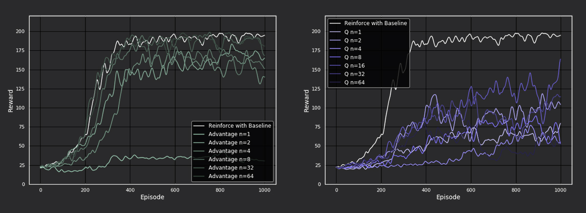
Figure 8: Performance of higher n-step actor-critic methods on cartpole

Here we see that the advantage actor-critic methods with larger n-step values 32 and 64 perform better than the methods with the smaller n-step values. This time, we have found two n-step values that perform just as well as REINFORCE with baseline! For Q actor-critic methods, larger n-step values did not improve performance. An explanation for the positive effect of larger N on the performance could be that the algorithm performs like REINFORCE when the length of the episode is smaller than N (beginning of training), while when the episodes get longer (end of training) than N it is a bit more stable than REINFORCE because it makes use of bootstrapping.

Behavior

Cartpole

Figure 9: Behavior simulation in Cartpole environment

When visualizing the trained agents, we can observe some cool differences in behavior!

In the Cartpole environment, we see that at 1-step, the actor-critic agents typically fail to balance the pole for more than a few seconds and do not get a reward above 20. For n-step values greater than 1, the advantage actor-critic agents do a decent job of balancing the pole however they are inclined to move to one side while balancing it, which leads them to drop it. For Reinforce with baseline, the agent learns to balance the pole well by making small movements from left to right.

In the Lunar Lander environment, we see that the three agents have different approaches to landing the spaceship. The advantage actor-critic agent slowly lands by swaying from side to side (making use of the left and right engine), and learns to improve landing as the n-step increases, while the Q actor-critic agent comes crashing down quickly in all experiments. In general, the Reinforce agent has a more direct landing, but does not come to a halt after touching the surface and keeps firing its engines, which decreases reward. Check out the Figure 1 at the top of the page to see this comparison!

The Mountain Car environment is too challenging and does not result in different behaviors. All agents remain stuck in the valley, rolling from left to right.

Conclusion

All in all, our experiments demonstrate that increasing n-step values for Advantage actor-critic methods can lead to performance that is almost as good as REINFORCE with baseline but with less stability. Contrary to our hypothesis, tuning n did not increase performance compared to the basic REINFORCE with baseline algorithm. We can conclude that the best n-step value is dependent on the environment, which is something we did expect.

Although, our procedure showed success in (some/most) cases we generally observed a lot of variance in performance over different algorithms, environment and even random seeds. This shows us that policy gradients in deep reinforcement learning are complicated animals that demand considerable amounts of care taking and tuning. We can also emphasize findings presented by Ilyas et. al. 9 who state that in some prominent deep RL applications “performance depends heavily on optimizations not part of the core algorithm”, which are not necessarily described in the papers. These optimizations include reward scaling, learning rate annealing, orthogonal weight initialization and value clipping among others. We can only guess that some of these additional optimizations are, for example, the reason why the OpenAI baseline implementation of A2C (even with only one environment in parallel) consistently solves the MountainCar environment whereas our approach never managed to do so.

Code

Our code can be viewed here.

Citations

[1] High-dimensional continuous control using generalized advantage es-timation - https://arxiv.org/abs/1506.02438

[2] OpenAI Five - https://openai.com/blog/openai-five/

[3] Solving Rubik’s Cube with a Robot Hand - https://openai.com/blog/solving-rubiks-cube/

[4] A Closer Look at Deep Policy Gradients - http://gradientscience.org/policy_gradients_pt1/

[5] Deep Reinforcement Learning that Matters - https://arxiv.org/abs/1709.06560

[6] Reinforcement Learning: An Introduction - http://incompleteideas.net/book/RLbook2018.pdf

[7] OpenAI Baselines - https://github.com/openai/baselines

[8] Asynchronous Methods for Deep Reinforcement Learning - https://arxiv.org/abs/1602.01783

[9] Are Deep Policy Gradient Algorithms Truly Policy Gradient Algorithms? - https://arxiv.org/abs/1811.02553

Exploring Variance in N-Step Actor-Critic Methods

*David Biertimpel, *Claartje Barkhof, *Vicky Foing & *Alex Lindt

*University of Amsterdam | October 2019

Introduction

Policy Gradient Methods

Reinforce

Actor-Critic Methods

Policy Gradient Theorem

N-step bootstrapping

Methods

Experiments

Environments

Cartpole

Lunar Lander

Mountain Car

Experimental set-up & metrics

Architecture & hyper parameters

Results

Overall performances

Cartpole

Lunar Lander

Mountain Car

Comparing random seeds

Variance-bias debate

Larger N

Behavior

Conclusion

Code

Citations

David Biertimpel, Claartje Barkhof, Vicky Foing & Alex Lindt